Turnip Price Prediction
Imagine a market where, every Sunday, a certain trade good (in this case
turnips) becomes available for purchase. Throughout the following week (Monday to Saturday),
the market announces two daily buyback prices (one before 12 AM and another one after)
allowing traders to sell their turnips back at those rates. Naturally, an
 arises:
Based on observed buyback prices, when should one sell to maximize profits?
Answering this question is inherently challenging, and the quality and complexity of
any solution depend heavily on the information available about the specific market.
arises:
Based on observed buyback prices, when should one sell to maximize profits?
Answering this question is inherently challenging, and the quality and complexity of
any solution depend heavily on the information available about the specific market.
In this article, we will develop one such solution for the
turnip market
from the video game Animal Crossing: New Horizons, which, at a basic level, operates
just as described above. Thanks to data-mining conducted by
Ninji, we now understand precisely how buyback prices are determined. Although the process
remains random, this knowledge can be used by traders to gain a significant advantage.
For a comprehensive breakdown, check out
this PDF,
written by
Edricus. Alternatively, you can explore the
raw code
on GitHub. The ready to use tool I created can be found here:
Get rich quick with this simple trick!
High-Level Overview
From the information revealed by the data-mined code, we know that the buyback prices \(X:= (X_1,\ldots,X_{12})\), ordered Monday AM to Saturday PM, always follow one of four distinct patterns: "Decreasing" (DEC), "Small Spike" (SS), "Large Spike" (LS), and "Alternating" (ALT). Furthermore, each pattern can have a multitude of different variations. Most importantly however, there exists only a finite set of possible probability distributions that \(X\) can follow.
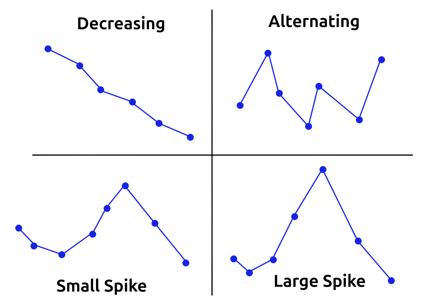
Possible buyback price pattern (placeholder).
Therefore, given observed buyback prices \(X\), we can utilize
Bayes' theorem
together with
the law of total probability
to determine the likelihood that each pattern variation \(V_k\) generated the observed
data.
\[ P(V_k | X) = \frac{P(X|V_k)P(V_k)}{P(X)} = \frac{P(X|V_k)P(V_k)}{\sum_i P(X |
V_i)P(V_i)}\]
These probabilities can then be used to rank all pattern variations, with the
highest-scoring ones providing the desired guidance on when to sell; as the structure
of each pattern indicates clear best-sell windows. That's the whole idea! Pretty easy,
right? However, this time around
Pattern Transitions
We begin by working on formulas for \(P(V_k)\). To select a pattern variation, the
game first chooses one of the four pattern types \(T_j\). After that it independently
chooses a specific variation \(V_k\) belonging to \(T_j\). Therefore, the probability
of a certain pattern variation being selected actually consists of two terms.
\[ P(V_k) = P(T_j) P(V_k|T_j) \]
The formulas for \(P(V_k|T_j)\) depend heavily on the structure of the pattern type
\(T_j\) and will be derived in the next section. The pattern probabilities \(P(T_j)\)
on the other hand are determined by a predefined
Markov chain
whose state depends on the previous week's pattern \(T^\prime_i\). The corresponding
transition matrix \(\mathbf{P}\) is defined as follows. For a more detailed
introduction to Markov chains, you can check out this other project of mine:
| \(T^\prime_i \to T_j\) | \(\texttt{DEC}\) | \(\texttt{SS}\) | \(\texttt{LS}\) | \(\texttt{ALT}\) |
|---|---|---|---|---|
| \(\texttt{DEC}\) | 0.05 | 0.25 | 0.45 | 0.25 |
| \(\texttt{SS}\) | 0.15 | 0.15 | 0.25 | 0.45 |
| \(\texttt{LS}\) | 0.20 | 0.25 | 0.05 | 0.50 |
| \(\texttt{ALT}\) | 0.15 | 0.35 | 0.30 | 0.20 |
Transition probabilities previous week's pattern \(T^\prime_i\) to this week's one
\(T_j\).
That being said, an immediate issue arises: How do we evaluate \(P(T_j) = P(T^\prime_i \to T_j)\) if \(T_i^\prime\) is unknown? Luckily, a bit of Markov chain theory can help with that. Consider, a row vector \(\pi_n\) representing the probability distribution of choosing any particular state (here the four pattern) at week \(n\). If the Markov chain is irreducible (i.e. every state can be reached from every other state) and aperiodic (i.e. it does not follow a fixed cycle), then a unique limit distribution \(\pi_\infty\) exists, satisfying \[ \pi_\infty \mathbf{P} = \pi_\infty\ \, \text{where}\ \sum_j (\pi_\infty)_j = 1\,. \] By definition, the limit distribution describes the overall probabilities of choosing any particular state and can therefore be used to evaluate \(P(T_j) = (\pi_\infty)_j\) whenever the previous week's pattern \(T^\prime_i\) is unknown. Next, we can easily compute \(\pi_\infty\) by rewriting the above equation as \((\mathbf{P}^T - I)\pi_\infty = 0\) with \(\pi_\infty \gets \pi_\infty^T\) and solving the resulting equation system numerically; for example, using NumPy in Python:
PY
                        def findStableState(transMat):
                            dim = transMat.shape[0]
                            target = transMat.T - np.eye(dim)

                            mat = np.vstack([target, np.ones(dim)])
                            vec = np.hstack([np.zeros(dim), 1])

                            return np.linalg.lstsq(mat, vec)[0]
Python code to find the limit distribution \(\pi_\infty\).
Running this code on our transition matrix \(\mathbf{P}\) yields the missing
transition probabilities if the previous week's pattern is unknown. Finally, one last
detail worth mentioning: If it is the player's first time buying turnips, the game
will always select a "Small Spike" variation, guaranteeing
| \(T^\prime_i \to T_j\) | \(\texttt{DEC}\) | \(\texttt{SS}\) | \(\text{LS}\) | \(\texttt{ALT}\) |
|---|---|---|---|---|
| \(\texttt{UN}\) | 0.148 | 0.259 | 0.247 | 0.346 |
Pattern Variations
Each of the four main patterns can be decomposed into a sequence of independent phases, whose lengths are what changes between corresponding variations. In fact, there are only three fundamental phase types: "Decreasing" (\(\texttt{DEC}\)), "Random" (\(\texttt{RAN}\)), and "Custom Spike A" (\(\texttt{CSTA}\)). Everything else is some combination of those. For example, the "Alternating" pattern quite literally just alternates between "Random" and "Decreasing" phases.
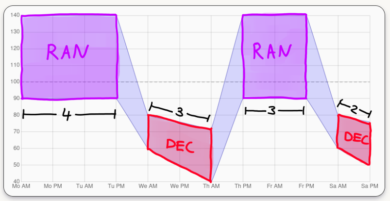
Range of a specific "Alternating" pattern variation
consisting of "Random" and "Decreasing" phases (placeholder).
consisting of "Random" and "Decreasing" phases (placeholder).
The exact procedures used to determine a pattern variation, that is, the lengths of its independent phases, can be inferred from the data-mined code and are described in great detail in the PDF by Edricus. The document also nicely explains when to sell during each pattern, allowing me to refer readers interested in those details to it. Here, I'll simply state the composition of the four main patterns as well as the corresponding formulas for \(P(V_k|T_j)\).
| pattern type \(\,T_j\) | composition variation \(\,V_k\) | \(P(V_k|T_j)\) |
|---|---|---|
| Decreasing | \(\texttt{DEC}\,\) (fundamental) | 1 |
| Small Spike | \(\texttt{DEC}_1, \texttt{RAN}, \texttt{CSTA} , \texttt{DEC}_2\) | \(\frac{1}{\#\texttt{DEC}_1} = \frac{1}{8}\) |
| Large Spike | \(\texttt{DEC}, \texttt{CSTB}, \texttt{RAN}\) | \(\frac{1}{\#\texttt{DEC}} = \frac{1}{7}\) |
| Alternating | \(\texttt{RAN}_1, \texttt{DEC}_1, \texttt{RAN}_2 , \texttt{DEC}_2, \texttt{RAN}_3\) | \(\frac{1}{14}\cdot\frac{1}{7-|\texttt{RAN}_1|}\) |
Pattern type, composition variation, and corresponding probabilities.
Note that "Custom Spike B" (CSTB) simply consists of five independent "Random" phases. Also note that whenever a formula includes a phase name in \(|\cdot|\), it should be replaced by that phase's length. If the phase name is preceded with a \(\#\), it should instead be replaced by the pattern's number of possible lengths for that phase. For example, in a "Small Spike" pattern, only \(\texttt{DEC}_1 \sim \mathcal{U}\{0,...,7\}\) is selected randomly. Every other phase either has a fixed length or is determined by the value of \(\texttt{DEC}_1\). Consequently, we obtain \[ \begin{align} P(V_k|T_j) &= P(\texttt{DEC}_1, \texttt{RAN}, \texttt{CSTA}, \texttt{DEC}_2 \,|\, \texttt{SS})\\[5px] &= \frac{1}{\#\texttt{DEC}_1} = \frac{1}{\#\{0,\ldots,7\}} = \frac{1}{8}\,. \end{align} \]
Basic Code Setup
As discussed, each pattern \(V_k\) can be decomposed into a sequence of independent
phases \(V_k^{(1)},\ldots,V_k^{(r)}\), where \(r\) denotes the sequence length of
\(V_k\). Consequently, both the data \(X \sim V_k\) and the probability\(P(X|V_k)\)
naturally decompose as follows.
\[ \begin{array}{c} \displaystyle X \sim V_k\ \Leftrightarrow
\mathop{\Huge\times}\limits_{i\leq r} X^{(i)} \sim \mathop{\Huge\times}\limits_{i\leq
r} V_k^{(i)} \\[5px] \displaystyle P(X|V_k) = \prod_{i\leq r}
P\big(X^{(i)}\big|V_{k}^{(i)}\big) \end{array} \]
We can mirror this structure in our code architecture by utilizing an abstract parent
class
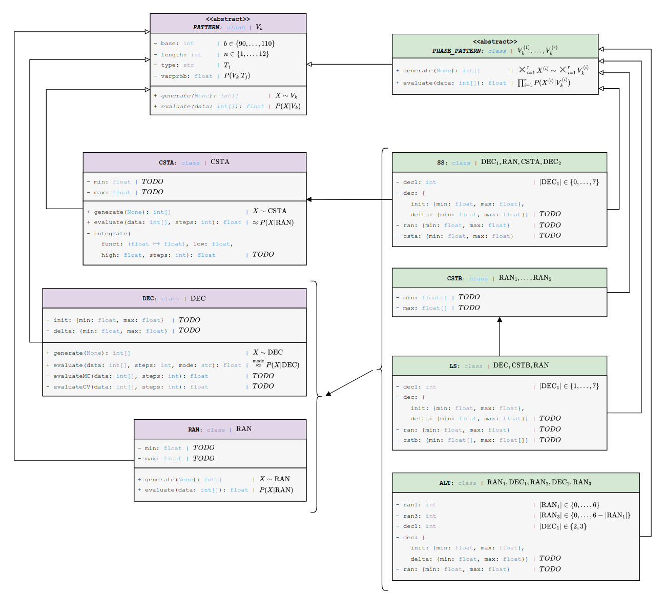
UML diagram for the PATTERN and PHASE_PATTERN class (TODO).
As always, keep in mind that the UML diagram above highlights only conceptually
important components. If you are interested in the complete implementation, you can
find the full code on
GitHub. As shown in the UML, the non-abstract classes extending
In the next sections we will be focused on first deriving the math behind, and
subsequently implementing, the
JS
                        // corresponds to (X^(1),...,X^(r)) ~ (V_k^(1),...,V_k^(r))
                        PHASE_PATTERN.generate = function() {
                            return this.phases.reduce((prices, phase) =>
                                prices.concat(phase.generate()), []);
                        }

                        // corresponds to P(X|V_k) = P(X^(1)|V_k^(1))*...*P(X^(r)|V_k^(r))
                        PHASE_PATTERN.evaluate = function(data) {
                            const copy = [...data]; // copy data before splicing
                            return this.phases.reduce((prob, phase) =>
                                prob * phase.evaluate(copy.splice(0, phase.length)), 1);
                        }
Implementations of generate and evaluate functions for PHASE_PATTERN.
We will skip the
RAN Phase
Earlier we stated that the "Random" phase is not decomposable; however, this is
 . In fact, \(X \sim \texttt{RAN}\) amounts to \(X = (X_1,\ldots,X_n)\), where
\[X_i = \big\lceil b R_i \big\rceil ,\;\; R_i \overset{iid}{\sim}
\mathcal{U}\big[\texttt{min},\,\texttt{max}\big] \,. \]
Therefore, a "Random" phase of length \(n\) can technically be decomposed into \(n\)
independent "Random" phases of length \(1\). In practice however, it is best not to do
so. Next, let \(A_i = \{k_i\}\) correspond to an observation \(k_i \in \mathbb{Z}\),
and let \(A_i = \mathbb{Z}\) denote an unobserved value. By defining
\[lA_i := \begin{cases} \Big[\frac{k_i-1}{b},\,\frac{k_i}{b}\Big], & A_i =
\{k_i\}\\[5px] \big[\texttt{min},\,\texttt{max}\big], & A_i = \mathbb{Z} \end{cases}\]
we can express the probability distribution of \(X\) in terms of the underlying rates
\(R\). Try to get used to this approach now, as the other two phases will be treated
in much the same way. The main complication is that, in those cases, the \(R_i\) are
no longer independent. Clearly we get
\[ P(X=k\,\big|\,\texttt{RAN}) \;\ = \prod_{i \,:\, A_i \neq \mathbb{Z}} P\big(R_i \in
l\{k_i\}\big) \,.\]
To evaluate the inner terms, set \(H := \big[\texttt{min},\,\texttt{max}\big]\), then
integrate the PDF \(f_R \sim \mathcal{U}(H)\) over \(l\{k_i\}\).
\[ P\big(R_i \in l\{k_i\}\big) = \int_{l\{k_i\}} f_R \,d\lambda = \frac{1}{|H|} \int
I_H I_{l\{k_i\}}\,d\lambda = \frac{|H \cap l\{k_i\}|}{|H|} \]
This is a
. In fact, \(X \sim \texttt{RAN}\) amounts to \(X = (X_1,\ldots,X_n)\), where
\[X_i = \big\lceil b R_i \big\rceil ,\;\; R_i \overset{iid}{\sim}
\mathcal{U}\big[\texttt{min},\,\texttt{max}\big] \,. \]
Therefore, a "Random" phase of length \(n\) can technically be decomposed into \(n\)
independent "Random" phases of length \(1\). In practice however, it is best not to do
so. Next, let \(A_i = \{k_i\}\) correspond to an observation \(k_i \in \mathbb{Z}\),
and let \(A_i = \mathbb{Z}\) denote an unobserved value. By defining
\[lA_i := \begin{cases} \Big[\frac{k_i-1}{b},\,\frac{k_i}{b}\Big], & A_i =
\{k_i\}\\[5px] \big[\texttt{min},\,\texttt{max}\big], & A_i = \mathbb{Z} \end{cases}\]
we can express the probability distribution of \(X\) in terms of the underlying rates
\(R\). Try to get used to this approach now, as the other two phases will be treated
in much the same way. The main complication is that, in those cases, the \(R_i\) are
no longer independent. Clearly we get
\[ P(X=k\,\big|\,\texttt{RAN}) \;\ = \prod_{i \,:\, A_i \neq \mathbb{Z}} P\big(R_i \in
l\{k_i\}\big) \,.\]
To evaluate the inner terms, set \(H := \big[\texttt{min},\,\texttt{max}\big]\), then
integrate the PDF \(f_R \sim \mathcal{U}(H)\) over \(l\{k_i\}\).
\[ P\big(R_i \in l\{k_i\}\big) = \int_{l\{k_i\}} f_R \,d\lambda = \frac{1}{|H|} \int
I_H I_{l\{k_i\}}\,d\lambda = \frac{|H \cap l\{k_i\}|}{|H|} \]
This is a
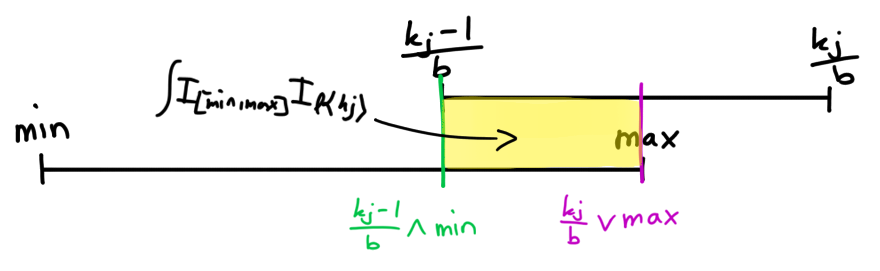
\(H\) and \(l\{k_i\}\) overlapping each other (placeholder).
Similarly the condition \(H \cap l\{k_i\} \neq \emptyset\) can be expressed as conditions to the bounds of the intervals \(H\) and \(l\{k_i\}\). Finally, setting \(a \vee b := \min(a,b)\) and \(a \wedge b := \max(a,b)\), not to be confused with \(\texttt{min}\) and \(\texttt{max}\), we get \[|H \cap l\{k_i\}| = \bigg[\bigg( \frac{k_i}{b} \vee \texttt{max} \bigg) - \bigg( \frac{k_i-1}{b} \wedge \texttt{min} \bigg) \bigg]\, I\bigg\{\frac{k_i}{b} \geq \texttt{min},\, \frac{k_i-1}{b} \leq \texttt{max}\bigg\} \,.\] To calculate \(P(X=k\,|\,\texttt{RAN})\) in code, we just need to directly implement the derived formula, then iterate over all given data points and multiply the results. If we encounter a data point for which the above indicator is zero, we can immediately stop the calculation and simply return zero. Likewise, if a data point is unobserved, we can immediately skip to the next one.
JS
                        RAN.evaluate = function(data) {
                            const { base, min, max } = this;

                            // corresponds to I{k/b >= min, (k-1)/b <= max}
                            const valid = (point) =>
                                point / base >= min && (point - 1) / base <= max;

                            let prob = 1;
                            for (let point of data) {
                                // missing datapoint: multiply by 1
                                // invalid datapoint: return 0
                                if (!point) continue;
                                if (!valid(point)) return 0;

                                // observed datapoint: multiply with P(R_j ∈ l{k_j})
                                const high = Math.min(point / base, max);
                                const low = Math.max((point - 1) / base, min);
                                prob *= (high - low) / (max - min);
                            }

                            return prob;
                        }
Evaluation function of "Random" phase directly implements derived formula.
CSTA Phase
The second phase we will discuss is the "Custom Spike A" phase. As before, let \(H := \big[\texttt{min},\,\texttt{max}\big]\) and define \(Q(m) := \big[ \texttt{min},\,m \big]\). Then \(X \sim \texttt{CSTA}\) means \(X = (X_1,X_2,X_3)\), where \[ \begin{array}{c} X_1 = \big\lceil b R \big\rceil - 1,\;\; X_2 = M,\;\; X_3 = \big\lceil b S \big\rceil - 1\\[2px] M \sim \mathcal{U}(H),\;\; R,S \overset{iid}{\sim} \mathcal{U}(Q(M)) \,. \end{array} \] Notice that the rates \(R,S\) now depend on the rate \(M\). In addition, both \(X_1\) and \(X_3\) now contain an extra "\(-1\)" term. Luckily, this is easy to fix later, allowing us to ignore it for now. With the same sets \(A\) and operator \(l\) as before, consider the following probability \[ \begin{align} & P\big( M \in lA_M, \, (R,S) \in lA_{R \times S} \big)\\[5px] &\qquad\overset{\star_1}{=} \int_{lA_M} f_M \int_{lA_{R \times S}} f_{(R,S)|M} \,d\lambda^2 \ d\lambda\\[5px] &\qquad \overset{\star_2}{=} \int_{lA_M} f_M \bigg( \int_{lA_R} f_{R|M}\,d\lambda \int_{lA_S} f_{S|M}\,d\lambda \bigg)\ d\lambda\\[5px] &\qquad= \frac{1}{|H|} \int_{lA_M \cap H} \rho_R\rho_S\,d\lambda\ \ \ (\star) \end{align} \] where we used the law of total probability at \(\star_1\) and \(lA_{R \times S} = lA_R \times lA_S\) at \(\star_2\). The two inner integrals are essentially identical and evaluate exactly as already seen in the discussion of the \(\texttt{RAN}\) phase above. \[ \rho_R(m) := \int_{lA_R} f_{R|M=m} \,d\lambda = \frac{|Q(m) \cap lA_R|}{|Q(m)|}\ \ \ (\star\star) \] Note \(\rho_R,\rho_S\) analogous. The remaining integral at \((\star)\) can be nicely approximated using a Riemann sum. To this end, let \((x_k)_{j \leq n}\) be a grid on \(lA_M \cap H\) with step size \(\delta_n\). Then it holds \[ \sum_{j \leq n} (\rho_R\rho_S)(x_j)\,\delta_n \overset{n \to \infty}{\longrightarrow} \int_{lA_M \cap H} \rho_R\rho_S\,d\lambda \,.\] Finally, to translate from \(X\) to the underlying rates \(M,R,S\) define \(qx := x + 1\) and replace \(A_R \gets qA_R\) and \(A_S \gets qA_S\). This compensates for the "\(-1\)" offsets in the definitions of \(X_1\) and \(X_3\), yielding \(P(X=k\,|\,\texttt{CSTA}) = P( M \in lA_M, \, (R,S) \in lA_{R \times S})\) as desired. To implement this in code, we begin by defining the indicator appearing in \((\star\star)\), as well as a function for \(\rho_R\) and \(\rho_S\).
JS
                        // corresponds to I{k/b >= min, (k-1)/b <= m}
                        const valid = (point, m) =>
                            point / base >= min && (point - 1) / base <= m;

                        const rho = (point, m) => {
                            // [CHECK FIRST] missing datapoint: return 1
                            // invalid datapoint or bad division: return 0
                            if (!point) return 1;
                            if (!valid(point, m) || m == min) return 0;

                            // observed datapoint: return rho(m)
                            const high = Math.min(point / base, m);
                            const low = Math.max((point - 1) / base, min);
                            return (high - low) / (m - min);
                        };
Implementation of \(\rho_R,\rho_S\) functions.
Next, we set up the integration by determining the bounds of the integration region
and defining the integrant \(x \mapsto (\rho_R\rho_S)(x)\). Note that the the shifts
\(A_R \gets qA_R\) and \(A_S \gets qA_S\) are implemented by adding \(1\) to the
points
JS
                        // corresponds to min(k_M/b, max) and max((k_M-1)/b, min)
                        const high = !!M ? Math.min(M / base, max) : max;
                        const low = !!M ? Math.max((M - 1) / base, min) : min;

                        // corresponds to integrand x ⟼ (ρ_Rρ_S)(x)
                        const fun = (x) => rho(R + 1, x) * rho(S + 1, x);
Integration bounds and integrand code.
Putting everything together, the
JS
                        CSTA.evaluate = function(data, steps = 50_000) {
                            const { base, min, max } = this;
                            const [R, M, S] = data;

                            // implemented as stated above
                            const valid, rho, low, high, fun;

                            // if integration region empty return prob 0
                            if (!!M && !valid(M, max)) return 0;

                            const approx = CSTA.integrate(fun, low, high, steps);
                            return approx / (max - min);
                        }
Evaluation function of "Custom Spike A" phase utilizing a Riemann sum.
DEC Phase (MC)
Oh boy did I get
We will begin by discussing the MC approach. For that, let \(H_1 := \big[\texttt{init.min},\,\texttt{init.max}\big]\) and \(Q := \big[\texttt{delta.min},\,\texttt{delta.max}\big]\). Then \(X \sim \texttt{DEC}\) is defined as \(X = (X_1,\ldots,X_n)\), where \[ \begin{array}{c} X_i = \big\lceil bR_i \big\rceil, \;\; R_{i+1} = R_i - \Delta_i\\[2px] R_1 \sim \mathcal{U}(H_1), \;\; \Delta_i \overset{iid}{\sim} \mathcal{U}(Q) \,. \end{array} \] We are interested in the probability \(P(R \in lA) = \int_{lA} f_R \,d\lambda^n\) where \(R = (R_1,\ldots,R_n)\) and \(lA := lA_1 \times \cdots \times lA_n\). Since \(R_{i+1}\) depends on \(R_i\) evaluating this integral directly quickly becomes unwieldy. Instead, we will find the probability distribution of \(R\), allowing us to come up with a clever way to approximate \(P(R \in lA)\). To this end, consider \(\Delta := (R_1,\Delta_2,\ldots,\Delta_n)\), whose components are independent, making it easy to find its PDF \[ \begin{align} &f_\Delta(h_1,s_2,\ldots,s_n) = f_1(h_1) \prod_{i \geq 2} f_Q(s_i)\\[5px] &\qquad = \frac{I\{h_1 \in H_1\}}{|H_1|} \prod_{i \geq 2} \frac{I\{s_i \in Q\}}{|Q|}\\[5px] &\qquad = \frac{I\big\{h_1 \in H_1,\, \forall i \geq 2 : s_i \in Q\big\}}{|H_1|\,|Q|} \end{align} \] where \(f_1 \sim \mathcal{U}(H_1)\) and \(f_Q \sim \mathcal{U}(Q)\). Next, we will use the PDF transformation theorem \((\star)\) to derive \(f_R\) from \(f_\Delta\). Consider a linear map \(T : \mathbb{R}^n \to \mathbb{R}^n,\, x \mapsto Tx\) given by the triangular matrix \[ T = \left[ \begin{smallmatrix} 1 \\ 1 & -1 \\ \vdots & \vdots & \ddots \\ 1 & -1 & \cdots & -1 \end{smallmatrix} \right],\ T^{-1} = \left[ \begin{smallmatrix} 1 \\ 1 & -1 \\ & \ddots & \ddots \\ & & 1 & -1\end{smallmatrix} \right]. \] It holds \(T\Delta = R\) as desired and \(\det T = (-1)^{n-1} \neq 0\), allowing us to apply the theorem. For \(h \in \mathbb{R}^n\) we obtain \(f_R\), which is guaranteed to be a PDF (this will be important in a bit), as \[ \begin{align} f_R(h) &\overset{\star}{=} f_\Delta\big(T^{-1}h\big)\, \underbrace{\big|\det T^{-1}h\big|}_{= |1 / \det T| = 1}\\[5px] &= \frac{I\big\{ h_1 \in H_1,\, \forall i \geq 2 : h_{i-1} - h_i \in Q \big\}}{|H_1||Q|} \,. \end{align} \] Notice that the above indicator defines a set \(B \subset \mathbb{R}^n\) and since all PDF's must integrate to \(1\), we further obtain \[ 1 = \int f_R \,d\lambda^n = \frac{1}{|H_1|\,|Q|} \int_B d\lambda^n = \frac{|B|}{|H_1|\,|Q|} \] showing that \(f_R(h) = I\{h \in B\}\, |B|^{-1}\) and consequently \(R \sim \mathcal{U}(B)\). This allows us to nicely approximate the desired probability. Consider \(\psi\) to be the ratio of \(lA \cap B\) in \(B\). It then holds \[ P(R \in lA) \overset{R \sim \mathcal{U}(B)}{=} \frac{|lA \cap B|}{|B|} = \frac{\psi\,|B|}{|B|} = \psi \,.\] Now consider \(Y^{(j)} \overset{iid}{\sim} \mathcal{U}(B)\) yielding \(I\{Y^{(j)} \in lA\} \overset{iid}{\sim} \mathcal{Bin}(1,\psi)\) by definition of \(\psi\). Hence we can construct the following estimator and apply the law of large numbers to get the asymptotic \[ \hat{\psi}_m := \frac{1}{m} \sum_{j \leq m} I\{Y^{(j)} \in lA\} \ \overset{m \to \infty}{\longrightarrow}\ P(R \in lA) \,. \] Finally, notice that \(Y^{(j)} = T^{-1}\Delta^{(j)}\) allowing us to easily generate \(Y^{(j)} \sim \mathcal{U}(B)\). And that's it! The most challenging part for me was realizing that the distribution of \(R\) could be obtained from the much simpler \(\Delta\). Once I knew that \(R \sim \mathcal{U}(B)\) I quickly had the discussed approximation down. To implement this in code, we begin by defining a function to sample \(\Delta^{(j)}\) as well as one to transform them via \(T^{-1}\).
JS
                        // corresponds to Δ = (R_1,Δ_2,...,Δ_n)
                        const sample = () => {
                            // corresponds to R_1 ~ U(H_1)
                            const sample = [UTIL.randFl(init.min, init.max)];

                            // corresponds to Δ_i ~ U(Q)
                            for (let i = 1; i < data.length; i++)
                                sample[i] = UTIL.randFl(delta.min, delta.max);

                            return sample;
                        };

                        // corresponds to T^(-1)Δ ~ U(B)
                        const transform = (sample) => {
                            // corresponds to (T^(-1)h)_1 = h_1
                            let result = [sample[0]];

                            // corresponds to (T^(-1)h)_i = h_(i-1) - h_i
                            for (let i = 1; i < sample.length; i++)
                                result.push(result[i - 1] - sample[i]);

                            return result;
                        };
Sampling \(\Delta^{(j)}\) by pulling components from \(H_1\) and \(Q\)
and transforming a \(\Delta^{(j)}\) sample into \(Y^{(j)} \sim \mathcal{U}(B)\) via \(T^{-1}\).
and transforming a \(\Delta^{(j)}\) sample into \(Y^{(j)} \sim \mathcal{U}(B)\) via \(T^{-1}\).
Next, we need to implement \(I\{Y^{(j)} \in lA\}\) i.e. check if \(Y^{(j)}_i \in lA_i\) for all \(i\) where \(l\{k_i\}\) is as before and \(lA_i = H_i\) is the smallest interval such that \(R_i \in H_i\) almost surely.
JS
                        // corresponds to lA_i
                        const interval = (i) => !data[i]
                            // unobserved datapoint return H_i
                            ? [init.min - i * delta.max, init.max - i * delta.min]
                            // observed datapoint return l{k_i}
                            : [(data[i] - 1) / base, data[i] / base];

                        // corresponds to I{Y ∈ lA}
                        const valid = (rates) => rates.every((rate, i) => {
                            const [low, high] = interval(i);
                            return rate >= low && rate <= high;
                        });
Implementation of indicator \(I\{Y^{(j)} \in lA\}\) by checking each component.
Putting everything together, the
JS
                        DEC.evaluateMC = function(data, steps = 50_000) {
                            // if no data observed, return prob = 1
                            if (data.every((x) => !x))
                                return { hits: steps, ratio: 1 };
                            const { base, init, delta } = this;

                            // implemented as stated above
                            const sample, transform, valid;

                            // approximate phi by LLN
                            let hits = 0, n = steps;
                            while (n-- > 0) {
                                const sequence = transform(sample());
                                if (valid(sequence)) hits += 1;
                            }

                            return { hits, ratio: hits / steps };
                        }
Evaluation function of "Decreasing" phase utilizing Monte Carlo Estimation.
DEC Phase (RC)
While the MC approach provides an elegant asymptotic solution in theory, it
unfortunately suffers from several practical limitations. For starters, it is
inherently non-deterministic, meaning that evaluating
\(P(X\,|\,\texttt{DEC}_{\texttt{MC}})\) for the same data \(X\) twice may yield
slightly different results. Of course, this can be mitigated to some extend by running
a longer estimation (i.e. checking more \(I\{Y^{(j)} \in lA\}\)), however even with
multithreading
 remains little more than a band-aid fix.
More importantly, the method appears to degenerate quite aggressively with higher dimensionality (i.e. longer phases to check) and rare boundary cases (i.e. sequences that lie near the edge of possibility). I suspect that probing for \(lA\) simply using \(Y^{(j)} \sim \mathcal{U}(B)\ iid\) may not be sufficient in practice, even thought the theory clearly doesn't care. A possible fix would therefore need to implement a more sophisticated probing strategy, such as adaptive grids or similar techniques.
We will now cover the RC approach, which I discovered online and whose theoretical foundation is given by the Chapman-Kolmogorov equation. However, I believe it is more approachable to develop the tools we actually need ourselves. To that end, let \(X_1,\ldots,X_n\) be independent and satisfy \[ X_k \sim \mu_k, \;\; Y_k := Y_{k-1} + X_k, \;\; Y_1 := X_1 \,. \] We are interested in the distribution of the random walk \(Y = (Y_1,\ldots,Y_n)\). The key idea is based on the fact that \(Y_k = X_1 + \cdots + X_k\) is a sum of independent random variables. Therefore, its distribution can be obtained by convolving the distributions \(\mu_1,\ldots,\mu_k\).
Theorem. For a function \(f\), sets \(A_k\), and distributions \(\mu_k\) as above, define \(M_k f := f \cdot I_{A_k}\) and \(C_k f := f * \check{\mu}_k\). Then the recursion \(u_{k-1} = M_{k-1} C_k\, u_k\) with \(u_n = I_{A_n}\) yields \[ P(\forall k: Y_k \in A_k) = \int u_1(x) \,\mu_1(dx) \,. \]
Before proving the theorem, it is helpful to understand the intuition behind it. The operator \(M_{k-1}\) encodes the constraint \(Y_{k-1} \in A_{k-1}\) into \(u_k\), while the operator \(C_{k}\) encodes the (reflected) distribution \(\check{\mu}_k\) of the increment \(X_k\). As the recursion concludes, all constraints and all distributions, except \(\mu_1\) have been encoded into \(u_1\). Therefore, the desired probability can be obtained by simply integrating \(u_1\) against \(\mu_1\).
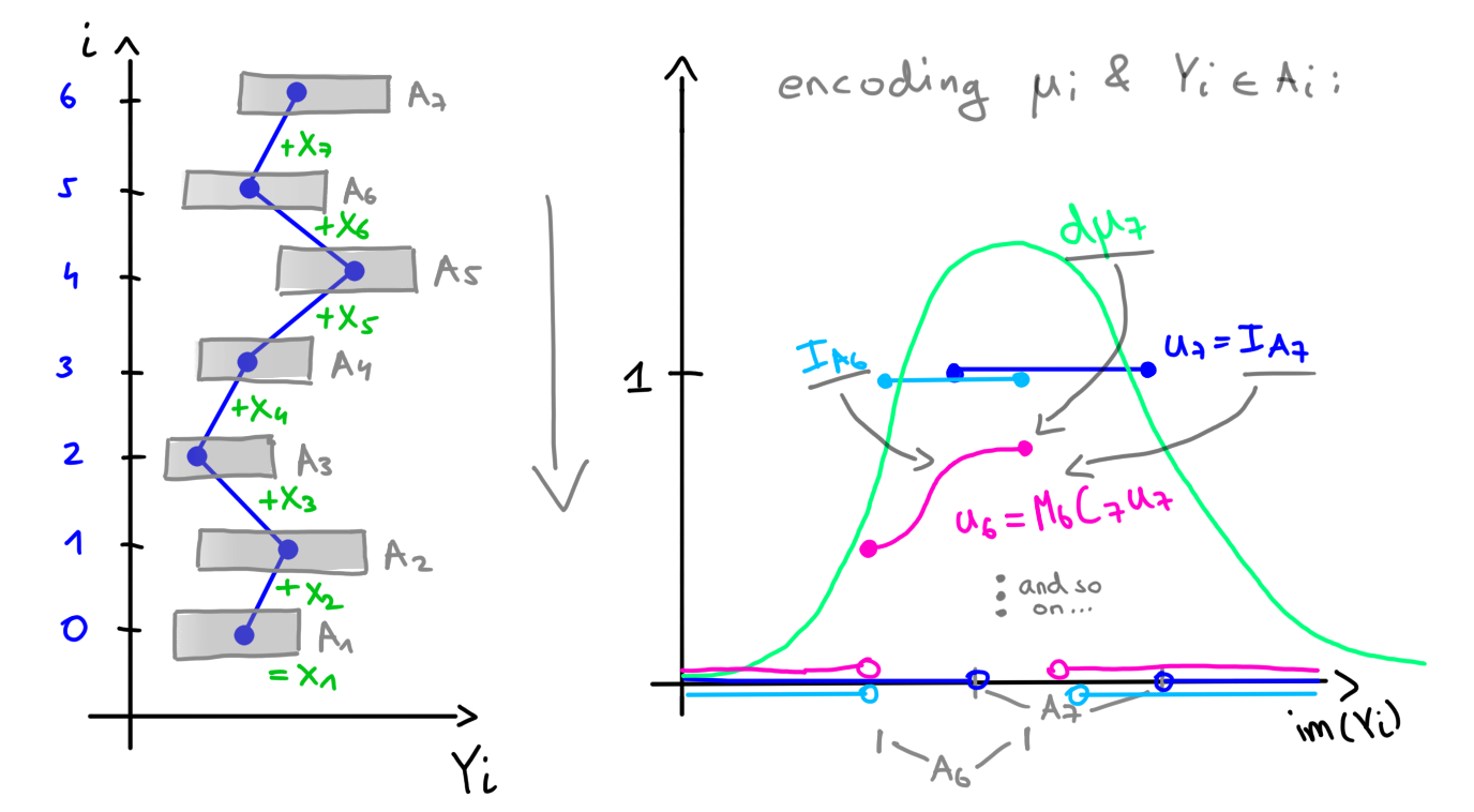
Encoding \(\mu_k\) and \(Y_k \in A_k\) into \(u_1\) (placeholder).
Proof.
To proof the theorem, we will need two main insights. First, since \(C_k\) convolves
with the reflected measure \(\check{\mu}_k(B) = \mu(-B)\), we can express the term
\(C_ku_k\) as follows.
\[ \begin{align} C_k u_k (x) &= (u_k * \check{\mu}_k) (x) = \int u_k(x-y)
\,\check{\mu}_k(dy)\\[5px] &= \int u_k(x+y) \,\mu_k(dy) = \int u_k(y) \,\mu_k(dy-x)
\quad (\star) \end{align} \]
Next, since \(Y_k = Y_{k-1} + X_k\) depends only on \(Y_{k-1}\), it is a markov
process with kernel \(\kappa_k(x_{k-1},A_k) = \mu_k(A_k-x_{k-1})\) \((\star\star)\).
Finally, define the distributions \(\nu_k \sim (Y_1,\ldots,Y_k)\), as well as the
notation \(\mathbf{A_k} := A_1 \times \cdots \times A_k\), \(\mathbf{dx_k} :=
dx_1,\ldots,dx_k\), and \(I_k(x) := I\{x \in A_k\}\). We can then repeatably use both
of these insights to proof the theorem.
\[ \begin{align} P(\forall k : Y_k \in A_k) &= \int_{\mathbf{A_n}}
\nu_n(\mathbf{dx_n}) \overset{(\star\star)}{=} \int_{\mathbf{A_n}} \mu_n(dx_n-x_{n-1})
\,\nu_{n-1}(\mathbf{dx_{n-1}}) \\[5px] &= \int_{\mathbf{A_{n-2}}}
\underbrace{I_{n-1}(x_{n-1}) \int u_n(x_n)\,
\mu_n(dx_n-x_{n-1})}_{\overset{(\star)}{=}\, M_{n-1} C_nu_n(x_{n-1})
\,=\,u_{n-1}(x_{n-1})} \,\nu_{n-1}(\mathbf{dx_{n-1}}) \\[5px]
&\overset{\circlearrowright}{=} \int \underbrace{I_1(x_1) \int u_2(x_2)
\mu_2(dx_2-x_1)}_{\overset{(\star)}{=}\, M_1C_2u_2(x_1) \, = \, u_1(x_1)} \,
\nu_1(\mathbf{dx_1}) = \int u_1(x_1)\,\mu_1(dx_1) \end{align} \]
Note that the above algebra assumes \(n > 2\), the cases \(n = 1,2\) are trivial to
check.
Observe that the above theorem describes an algorithm on how to calculate the desired probability. To this end, assume \(\alpha := \inf \bigcup_kA_k\) and \(\beta := \sup \bigcup_kA_k\) finite, yielding the grid \[x_i := \alpha + \Big(i + \frac{1}{2}\Big) \Delta x \,,\quad \mathcal{C}_i := \Big(x_i \pm \frac{\Delta x}{2}\Big]\] where \(\Delta x := \frac{\beta-\alpha}{m}\) and \(i = 0,\ldots,m-1\). By partitioning the interval \([\alpha, \beta]\) into \(\bigsqcup_j \mathcal{C}_j\) and setting \(u_k\big|_{\mathcal{C}_j} \equiv u_k(x_j)\) constant on each cell \(\mathcal{C}_j\) we obtain the approximation \[ \begin{align} C_ku_k(x_i) &\overset{(\star)}{=} \int_\alpha^\beta u_k(x)\,\mu_k(dx-x_i)\\[5px] &\approx \sum_{j \lt m} \underbrace{u_k(x_j)}_{=:\,u^{(k)}_j}\,\underbrace{\mu_k(\mathcal{C}_j-x_i)}_{=:\, W^{(k)}_{ij}} = \big(W^{(k)} u^{(k)}\big)_i \,. \end{align} \] By defining \(W^{(k)}_{ij}\) and \(u_j^{(k)}\) as above, we can express the operation \(C_k u_k = W^{(k)}u^{(k)}\) in terms of a simple matrix multiplication. Finally, the elements of \(W^{(k)}\) can be expressed by the CDF \(F_k(x) := \mu_k(-\infty,x]\) as follows. \[ W^{(k)}_{ij} = \mu_k(\mathcal{C}_j-x_i) = F_k\Big(x_j-x_i+ \frac{\Delta x}{2}\Big) - F_k\Big(x_j-x_i - \frac{\Delta x}{2}\Big) \] We are now ready to describe the complete algorithm computing \(P(\forall k : Y_k \in A_k)\). It is presented using mathematical pseudo code, as it is still part of the theoretical development.
PSEUDO
\[ \renewcommand{\bullet}{\;\;\, {\scriptstyle\blacktriangleright} \quad}
\newcommand{\bullett}{\quad \quad \quad {\scriptstyle\blacktriangleright} \quad}
\begin{array}{l|c} u \gets \texttt{array length } m\\[5px] \texttt{for } i =
0,\ldots,m-1: & \color{green}{\mathcal{O}(m)}\\[5px] \bullet u[i] \gets u_n(x_i) =
I\{x_i \in A_n\} \\[20px] \hline \texttt{for } k = n-1, \ldots, 1 : \\[5px] \bullet
\texttt{calculate } W^{(k+1)} & \color{red}{\mathcal{O}(m^2)}\\[5px] \bullet v \gets
\texttt{array length } m\\[5px] \bullet v \gets W^{(k+1)} u^{(k+1)} &
\color{red}{\mathcal{O}(m^2)}\\[5px] \bullet \texttt{for } i = 0,\ldots,m-1 : &
\color{green}{\mathcal{O}(m)}\\[5px] \bullett u[i] \gets I\{x_i \in A_k\}\,
v[i]\\[20px] \hline p \gets 0\\[5px] \texttt{for } i = 0,\ldots,m-1 : &
\color{green}{\mathcal{O}(m)}\\[5px] \bullet p \gets p +
u[i]\Big[F_1\Big(x_i+\frac{\Delta x}{2}\Big) - F_1\Big(x_i-\frac{\Delta
x}{2}\Big)\Big] \end{array}\]
Algorithm based on above theorem with runtime analysis.
You could implement the algorithm exactly like this and get a usable result. However, as highlighted in red, handling the matrix \(W^{(k+1)} \in \mathbb{R}^{m \times m}\) naively leads to subpar runtime performance. Of course I had to fix this! To that end, notice \(x_j - x_i = (j-i)\Delta x\) and therefore \[ W^{(k)}_{ij} = F_k\Big( \big(j-i+\tfrac{1}{2}\big) \Delta x \Big) - F_k\Big( \big(j-i - \tfrac{1}{2}\big) \Delta x \Big) =: w^{(k)}_{j-i} \,. \] Hence, \(W^{(k)}_{ij}\) depends only on the difference \(j-i\) and takes at most \(2m-1\) unique values, reducing its calculation time to \(\mathcal{O}(m)\). Next, we will rewrite the approximation term for \(C_ku_k(x_i)\) as the discrete convolution between \(u^{(k)}\) and \(\check{w}^{(k)}\). \[ C_ku_k(x_i) \approx \sum_{j \lt m} u^{(k)}_j w_{j-i}{(k)} \overset{\star}{=} \sum_{j \in \mathbb{Z}} u_j^{(k)} \check{w}_{i-j}^{(k)} = (u^{(k)}*\check{w}^{(k)})_i\] At \(\star\) we extended both vectors to sequences over \(\mathbb{Z}\) by padding them with zero. To exploit this structure recall that \(\mathcal{F}(f * g) = \mathcal{F}f \cdot \mathcal{F}g\) where \(\mathcal{F}\) is the Fourier transform. The right-hand side of this identity can trivially be computed in \(\mathcal{O}(m)\) time. Moreover, there exists an algorithm called the "Fast Fourier Transform" (FFT), computing both \(\mathcal{F}f\) and \(\mathcal{F}^{-1}f\) in \(\mathcal{O}(m \log m)\) time. Consequently, it is faster to Fourier transform \(u^{(k)}, \check{w}^{(k)}\), multiply them pointwise, and inverse Fourier transform the result, than it is to simply compute \(W^{(k)}u^{(k)}\) directly.
PSEUDO
\[ \renewcommand{\bullet}{\;\;\, {\scriptstyle\blacktriangleright} \quad}
\newcommand{\bullett}{\quad \quad \quad {\scriptstyle\blacktriangleright} \quad}
\begin{array}{l|c} \texttt{for } k = n-1, \ldots, 1 :\\[5px] \bullet \texttt{calculate
} \check{w}^{(k)} & \color{green}{\mathcal{O}(m)} \\[5px] \bullet \check{w}^{(k)},
u^{(k)} \gets \mathcal{F}\check{w}^{(k)}, \mathcal{F}u^{(k)} &
\color{orange}{\mathcal{O}(m \log m)}\\[5px] \bullet v \gets \texttt{array length }
m\\[5px] \bullet v \gets \mathcal{F}^{-1} (\check{w}^{(k)} \cdot u^{(k)}) &
\color{orange}{\mathcal{O}(m \log m)}\\[5px] \bullet \texttt{for } i = 0,\ldots,m-1 :
& \color{green}{\mathcal{O}(m)}\\[5px] \bullett u[i] \gets I\{x_i \in A_k\}\, v[i]
\end{array}\]
Achieving quasi-linear runtime performance using FFT.
Finally, we are ready to apply the developed theory. I've decided against showing the JS code as before, since we already stated the algorithm in pseudo-code above and I feel like it would add nothing new. However, I'll go over some details arising from our exact problem.
Recall the setup of offered prices \(X_i = \big\lceil bR_i \big\rceil\) with underlying base rates \(R_{i+1} = R_i - \Delta_i\) where \(R_1 \sim \mathcal{U}(H_1)\) and \(\Delta_i \sim \mathcal{U}(Q)\, iid\). Here \(R = (R_1,\ldots,R_n)\) is the discussed random walk and \(P(R \in lA)\) is the probability of interest. Also we get \(\alpha = \min (lA_n)\) and \(\beta = \max (lA_1)\), since \(R_{i+1} \lt R_{i}\) by definition. The CDF \(F\) of a uniform distribution over an interval \([a,b]\) is given by \[F(x) = \begin{cases} 0 & x \leq a\\ \frac{x-a}{b-a} & a \lt x \lt b\\ 1 & b \leq x \end{cases} \,.\] Note that there are only two unique CDF's \(F_1 \sim \mathcal{U}(H_1)\), corresponding to \(R_1\), and \(F_2 \sim \mathcal{U}(Q)\), corresponding to \(\Delta_i\, iid\). Therefore, the algorithm only needs one unique kernel vector \(w^{(1)}\).
Performance Comparison
With all that extra work done, one naturally wonders: Was it actually worth it? Well, let's find out. For starters, the new RC method is deterministic and, unlike the MC approach, does not appear to degenerate with higher dimensions nor rare edge cases. Thats good, but how does it compare to the original MC method in terms of convergence rate and runtime performance?
To answer this, I generated 1,000 random "Decreasing" sequences of medium length and evaluated each using both methods for increasing values of \(m\) (i.e. the size of the random MC sample, or the number of RC grid divisions). For each evaluation I recorded the error (i.e. the deviation of the evaluation from the "true" one computed by the RC method using 50,000 grid divisions) and the runtime.
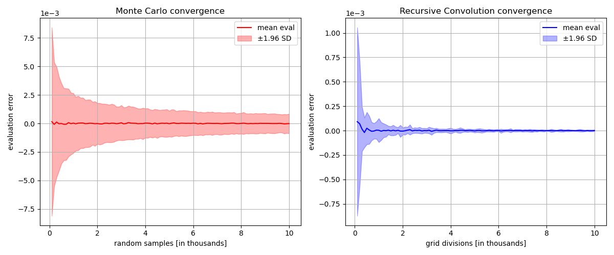
Convergence comparison between MC and RC methods (narrower is better).
Plotting the mean evaluation error together with the \( 95\%\) confidence intervals (mean \(\pm\)1.96 standard deviations) for each value of \(m\) immediately reveals quite the difference in convergence quality. In particular, notice that the RC method effectively starts from a smaller error level than the MC method ever gets to (below \(10^{-3}\)). This difference can be seen even more clearly when directly comparing the uncertainty of the two methods through their standard deviations.
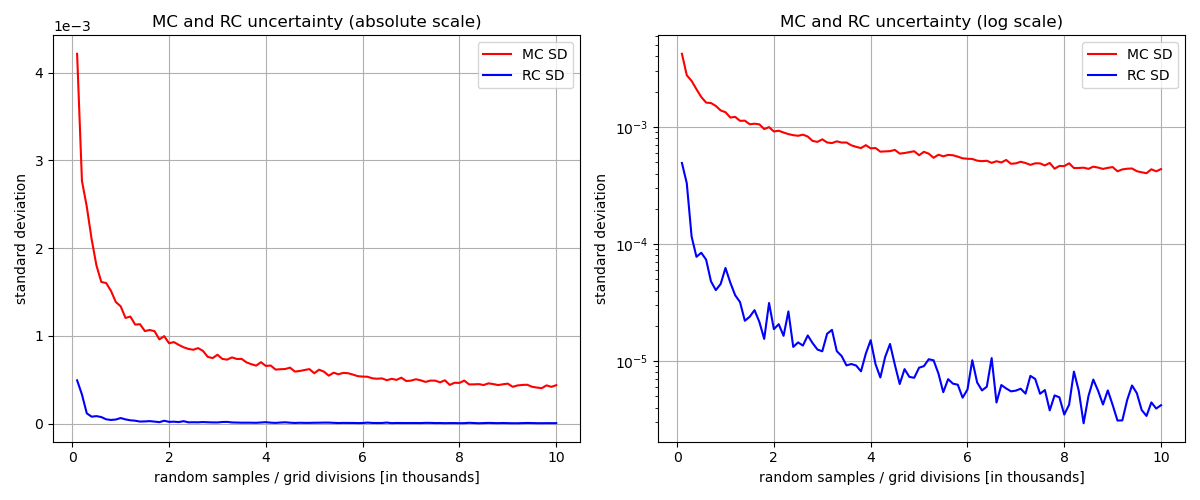
Uncertainty comparison between MC and RC methods (lower is better).
The RC method is the stronger method in terms of convergence and uncertainty. Its standard deviation decreases much more rapidly and reaches values up to two orders of magnitude smaller than those achieved by the MC method. But what about runtime performance? From the theoretical discussions above, we know that the MC method scales as \(\mathcal{O}(m)\), whereas the RC method scales as \(\mathcal{O}(m\log m)\). In practice the measured runtimes are as follows.
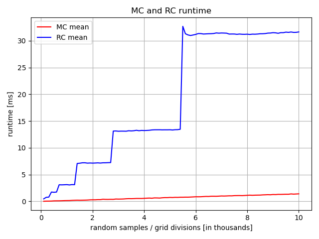
Runtime comparison between MC and RC methods (lower is better).
First, notice the staircase-like shape of the RC runtime. This behaviour comes from the convolution calculation \(u^{(k)}*\check{w}^{(k)}\) using the FFT algorithm. The length of a discrete convolution is given as the sum of the lengths of the individual vectors minus one. In our case we get \[ |u^{(k)}*\check{w}^{(k)}| = \underbrace{|u^{(k)}|}_{=\,m} + \underbrace{|\check{w}^{(k)}|}_{=\,2m-1} - 1 = 3m-2 \,. \] It is needed to zero-pad both vectors up to the length of the next power of two. Otherwise, the FFT computes the circular convolution rather than the linear one we require. Consequently, the jumps in the runtime graph correspond perfectly to the values of \(m\) s.t. \(3m-2\) exceeds the current power of two, forcing the convolution size to double. The small spike at \(m=5500\) is likely caused by my computer allocating additional memory for the just doubled convolution size.
At first glance, this graph seems to indicate a trade-off between accuracy and speed. However, to compare the two methods fairly, we should ask how long each takes to reach a reasonable accuracy level. For example, suppose we require an error level of at most \(\pm 0.1 \%\) with a certainty of at least \(95 \%\). For the RC method, we can see that is achieved essentially immediately. For the MC method, we can calculate the needed sample size and then linearly extrapolate (1.5ms for 10,000 samples) to estimate the total runtime. Recall the used estimator \[ \hat{\psi}_m = \frac{1}{m} \sum_{j \leq m} I\{Y^{(j)} \in lA\}\ \text{ with }\ I\{Y^{(j)} \in lA\} \sim \mathcal{Bin}(1,\psi) \,. \] We want \(P(|\hat{\psi}_m - \psi| \leq \epsilon) \geq 1 - \alpha\) for some \(\epsilon > 0\) and \(\alpha \in (0,1)\). For that, we can use the Central Limit Theorem (CLT) and the fact \((\star)\) that \(\Phi(-x) = 1 - \Phi(x)\) where \(\Phi \sim \mathcal{N}(0,1)\) CDF. \[ \begin{align} P\big(|\hat{\psi}_m - \psi| \leq \epsilon\big) &= P\Bigg( \underbrace{\frac{\sqrt{m}\,|\hat{\psi}_m-\psi|}{\sqrt{\psi(1-\psi)}}}_{\overset{\mathcal{D}}{\to}\,\mathcal{N}(0,1)} \leq \frac{\sqrt{m}\,\epsilon}{\sqrt{\psi(1-\psi)}}\Bigg)\\[5px] &\overset{\text{CLT}}{\approx} \Phi\Bigg( \frac{\sqrt{m}\,\epsilon}{\sqrt{\psi(1-\psi)}}\Bigg) - \Phi\Bigg(- \frac{\sqrt{m}\,\epsilon}{\sqrt{\psi(1-\psi)}} \Bigg) \\[10px] &\overset{(\star)}{=} 2\Phi\Bigg( \frac{\sqrt{m}\,\epsilon}{\sqrt{\psi(1-\psi)}} \Bigg) - 1 \end{align} \] Since \(\psi \in (0,1)\) is unknown we have to use the fact that \(\psi(1-\psi) \leq 1/4\), leading to \(\sqrt{m}\,\epsilon \,/ \sqrt{\psi(1-\psi)} \geq 2 \sqrt{m}\,\epsilon\), and since every CDF is non-decreasing we further get \[2\Phi\Bigg( \frac{\sqrt{m}\,\epsilon}{\sqrt{\psi(1-\psi)}} \Bigg) - 1 \geq 2\Phi\big(2 \sqrt{m}\,\epsilon\big) - 1 \overset{!}{\geq} 1-\alpha \,,\] which can be solved by using the inverse CDF \(u_{p} := \Phi^{-1}(p)\) for \(p \in (0,1)\) to obtain \[ m \overset{!}{\geq} \frac{1}{4}\Bigg( \frac{u_{1-\alpha/2}}{\epsilon} \Bigg)^2 \,. \] With \(\alpha = 0.05\) and \(\epsilon = 0.001\), corresponding to a target accuracy of \(\pm 0.1\%\) with at least \(95\%\) confidence, this yields \(m \approx 10^6\), or roughly one million samples! Based on the runtime extrapolation above, this would take \(150\text{ms}\) to run, which is orders of magnitude worse than the RC runtimes considered above. Thus, for realistic target accuracies, the deterministic RC method reaches the desired precision orders of magnitude faster than Monte Carlo despite its worse theoretical scaling behaviour.
Final Thoughts
This project turned out to be quite the challenge, especially due to the significant difficulty jump around the point where I needed decent methods for evaluating the three base phases. I'm really glad I pushed through it though, because I think the final result turned out quite impressive.
Of course, I'm neither the first nor the last person to build a turnip price prediction tool. One of the best-known example is Turnip Prophet, which I frequently used to compare predictions to. What's cool is that that project has over 60 contributors, whereas I did all of the work described above by myself. I'm definitely a little proud of that :) As always if you have any questions or found some mistake, feel free to contact me.